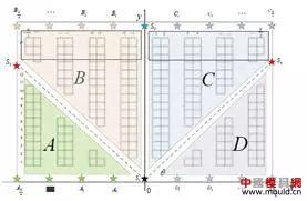
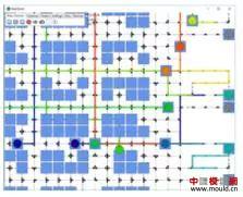
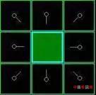
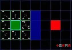
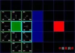
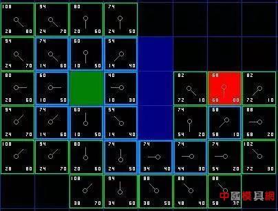
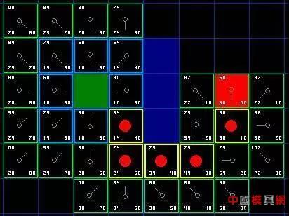
In practical applications, multiple AGV collaborative completion orders in a warehouse are indispensable parts, and the simultaneous path planning in the process of multiple AGV robots co-transport requires a certain algorithm to support. In this paper, multiple AGVs in a warehouse. The algorithm is researched in the direction of path planning, and its principle and implementation are analyzed and introduced. 2. Analysis First of all, our background is set in the logistics warehouse, which analyzes the specific task details such as warehousing, picking, and outbound in the warehouse to understand the scenes faced by our AGV. The traditional method generally adopts a static shelf. When the goods are transported to the designated shelf, the goods are manually put into the warehouse. When the goods are picked, the goods corresponding to the designated shelf picking order are manually packed out of the warehouse. After the introduction of the AGV, the mode will occur. Change, we will plan the designated storage area and picking area in the warehouse. AGV will dynamically transport the shelves containing the order to the picking area, wait in line for manual or robotic arm picking to the specified order picking basket, and complete the picking. Then transport the rack to the designated location. Therefore, after the introduction of AGV, the problem we face is to maximize efficiency, how to avoid congestion and collisions in multiple AGVs, how to plan a better walking route for each AGV, and how to make each AGV cost the least. To complete more tasks will be the focus of this article. 3. Problem disassembly In order to make multiple robots optimal in road planning, it is only necessary to consider the driving route of other cars when planning a single car, and then select an optimal driving plan. In addition, unlike outdoor scenes, we plan the car path in the warehouse, the entire road can be designed, so our problem can be disassembled as: (1) The design of roads in the warehouse; (2) Obtaining the route driving state of other cars; (3) Define possible road congestion; (4) Planning the shortest path; (5) Traffic control. 3.1 Road design in the warehouse Some common road designs are shown in Figure 1 and Figure 2. According to the actual application scenario, the factors considered include the structure of the warehouse, the type of goods, etc., and the optimal design is selected according to the actual test or simulation. Figure 1: V-shaped road design Figure 2: Tic Tac Toe Design 3.2 Obtaining the driving status of other cars In order to achieve global path planning, the position and running state of the car must be obtained at each moment, so a stable communication system must be established with the car. Generally, the wireless LAN is used to establish a connection with TCP, and a suitable WIFI channel is selected to ensure the car. Robust communication with the global path planning system. 3.3 Defining possible road congestion After the road planning of the warehouse is completed, the first factor to consider is the possible road congestion. Generally, the trolleys are walking straight in the warehouse. When they need to turn, they must stop at the original place. After the rotation is 90° or 180°, they will continue to walk straight. So every turn has a chance to cause current road congestion. In addition, when the traffic volume of the same road is large, it will also cause road congestion. In addition, there are three common possibilities for road congestion, such as turning, meeting and traffic flow. 3.4 Planning the shortest path Shortest path planning is the core of global path planning. To get from one location on the map to another, with obstacles in the middle and considering possible road congestion, a path search algorithm must be used to find the initial point to the target point. One of the shortest paths, the common search path algorithms are breadth-first algorithm, depth-first algorithm, Dijkstra algorithm, A* algorithm, etc. The breadth-first algorithm and the depth-first algorithm are applied to the tree structure to solve the shortest path or the minimum weight. The Dijkstra algorithm is generally used to solve the shortest path, and the A* algorithm is the most effective direct search method for solving the shortest path in the static road network. Each algorithm has its application scenario. For our global path planning scenario, our map is easier to convert into a raster map, and the A* algorithm has obvious advantages in searching for the shortest path on the raster map, and it is convenient to modify. Coupled with the consideration of our road congestion scenario, we use the A* algorithm as the preferred shortest path algorithm to analyze the global path planning. 3.5 Traffic Control Traffic control is mainly applied to meeting and co-current scenes. On the one hand, in order to avoid vehicle collisions, on the other hand, intersections are more common. If the treatment is not good, the vehicle will be deadlocked, the vehicles will wait for each other, and the task will not be completed. The core algorithm of planning, the common car scene is shown in Figure 3. Figure 3: Intersection car 4. Core algorithm implementation The core of the path planning algorithm is mainly the shortest path planning and traffic control. Here, a short path planning algorithm and traffic control algorithm are analyzed, and a complete global path planning algorithm is designed. 4.1 A* algorithm planning shortest path The A* algorithm is similar to the search for the optimal tree in graph theory. It is usually the cost of selecting a path for a path. There is always one path in all available paths, which is the least expensive compared to any other passable path. . When searching for the best path in graph theory, the path cost of each strip is known and fixed, but when solving the best path with A* algorithm, it goes along different paths, although it is the same node, its cost may be different. This is the essence of heuristic pathfinding. When using this method, the actual problem is first abstracted, and the elements in the problem are represented in the form of a matrix, including the starting position, the position of the target point, and the obstacles that appear. We will gradually find that in the aspect of path finding, the actual problems are abstractly represented by a matrix, and then the pathfinding process is realized by simulating the operation of the matrix. The basic idea is that the starting point is centered, and the 8 points in the immediate vicinity are pointed to it by the pointer, and the best waypoint is selected in the surrounding points and the surrounding point of the pointer is not established. , which is explained later in the article) by pointing the pointer to it, and selecting the best path point and then finding the way around the point until there is a target point in the surrounding point where the point is found, so that the searched path is connected one by one by the pointer. Finally, by outputting these points is the path to find. In the following, the pathfinding process of the A* algorithm is gradually analyzed through the following aspects: (1) Abstracting the actual problem into a matrix representation The abstracted matrix is ​​shown in Figure 4, where the green area represents the starting point, the red area represents the target point, the middle blue area represents the obstacle (such as a mountain or river that cannot pass), and the black area represents the area where the path can be generated. (2) Find the next node centering on the starting point As shown in FIG. 5, the eight points closely adjacent to the starting point are the next points that can be found on the path, and the intermediate current point is in the form of a pointer as the parent of the neighboring points. . For these 8 points, which point should be chosen as the next starting point for pathfinding, two lists are created in the A* algorithm, one is the open list (the available point for storing all current points (except that the list is already closed) The point in the middle, the obstacle point)), the other is the close list (where the stored point has been stored, the point already in the closed list will not be checked again in the next pathfinding process, which also indicates the wayfinding The lines will not have the possibility of intersecting). (3) Select the next node Add the starting point to the close list, and no longer check it in the subsequent pathfinding process. Next, select one of the 8 points as the next path point. The principle of selection is to find the node with the least cost in the path. Its weight is represented by F, F=G+H Where G is the starting point from the starting point, along the path generated, the path to the specified square is spent; as shown in Fig. 6, the starting point is centered, and the neighboring points have 8 points in the up, down, left and right, diagonal directions. The distance between the upper and lower movement paths is 10, and the diagonal cost is √2*10, which is about 14. Where H represents the movement path from the current point to the end point of the path, calculated as the sum of the number of horizontal and vertical squares between the current point and the destination point, and then multiplies the result by 10. As can be seen from Fig. 7, the weight F of the point on the right side of the starting point is the smallest, so it is taken as the next path point. (4) Continue searching Remove the path point from the open list and add it to the close list. Check the 8 points immediately adjacent to this point (ignoring the points in the close list or not passable), add them to the open list, and if there are points that are not added to the open list, use the path point as the parent of such points And added to the open list. If all feasible immediate points are already in the open list, check whether the current path to each adjacent point is less expensive than the path from the previous path point to the immediate point. If not, nothing is needed. 8) From the original starting point to the immediately lower right point, according to the newly generated path G value: G1=10+10=20, and the original path G value G2=14, that is, the newly generated path G value is smaller than the original path The G values ​​are large, and their H values ​​are the same (for the same point). Therefore, the F value of the original path is smaller than the F value of the newly generated path, and no processing is performed, and the next path is continued. If it is, then change the parent node of the adjacent square to the currently selected square, indicating that the movement of the newly generated path is less expensive. (5) Repeat the previous search process until the end There are two cases in the end of the search process: one is to add the target point to the close list, the search ends normally, and the path is found. In another case, the target point is not found but the open list is already empty, meaning that the path from the starting point to the target point is not found and the search ends. The search process is shown in Figure 9. It can be seen that there is a pointer from the starting point to the target point pointing to a consistent path, and the A* algorithm is the searched path. Add a red dot to highlight the path point, which is a path from the starting point to the ending point. The entire pathfinding process is organized as follows: 1) The start grid is added to the open list; 2) Repeat the following work: a) Find the point with the lowest F value in the open list. We call it the current point; b) add it to the close list; c) for each of the next 8 squares * If it is not passable or already in the close list, skip it. The opposite is as follows: * If it is not in the open list, add it to it. Use the current point as the parent of this cell. Record the F, G and H values ​​of this point; * If it is already in the open list, it is better to check the new path with the G value. A lower G value means a better path. If so, change the parent node of this point to the current point and recalculate the G and F values ​​for this point. After the change, you need to reorder the open list by F value. If not, you don't need to do the work of changing the pointer to point and recalculating the G and F values. 3) Stop searching, divided into two cases: * When the target point is added to the close list, the path is found and the search ends normally; * The target point was not found, but the open list is empty. At this time, the appropriate path was not found and the search ended. 4) Save the path. Starting from the target point, the pointer along each point points to move until it returns to the starting point and outputs the path. 4.2 Traffic control based on the lock mechanism After the completion of the vehicle road planning, multiple cars will start to walk at the same time. The situation of multiple road cars will be inevitable. When the car is in the car, the vehicles will mainly follow, and the opposite direction, the intersection or the T-junction, when the vehicle is followed There will be sensors to avoid following collisions. In order to avoid collisions between the crossroads and the T-shaped roads, the car will adopt the lock mode, namely: (1) Each trolley takes one step and locks the two-step point that is about to walk in front; (2) When the car locks the grid and finds that the point of the map to be locked has been locked, the two cars negotiate to see which priority is higher, which one is ahead, and the other is waiting; (3) The car will be unlocked after passing, and when you wait, you can re-lock the point you are about to drive and continue to walk forward; (4) The loop always performs a lock operation at each step. 4.3 Global Path Planning When planning the current car route, plan the shortest path in consideration of road congestion to meet the overall planning result. Use the A* algorithm to check whether the new path is better with the G value. If the G value of the point of the path planned by the car is increased, the same path can be avoided as much as possible. In the same way, when the vehicle needs to turn, the G value of the next point is also increased, so that the planned path avoids turning as much as possible. Appear to achieve the highest overall efficiency and the optimal global path. Weapon Ir Laser,Laser Weapon Infrared,Weapon Laser With Pressure Switch,Laser Weapon Nantong Dinggo Optical Instrument Co.,Ltd , https://www.riflescopeofficial.com
